Thursday, 13. September 2012
Sep 13
After the official Visual Studio 2012 launch yesterday I think it’s a good idea to announce two new type providers which are based on the DGMLTypeProvider from the F# 3.0 Sample Pack.
Synchronous and asynchronous state machine
The first one is only a small extension to the DGMLTypeProvider by Tao. which allows to generate state machines from DGML files. The extension is simply that you can choose between the original async state machine and a synchronous version, which allows easier testing.

If you want the async version, which performs all state transitions asynchronously, you only have to write AsyncStateMachine instead of StateMachine.
State machine as a network of types
The generated state machine performs only valid state transitions, but we can go one step further and model the state transitions as compile time restrictions:

As you can see the compiler knows that we are in State2 and allows only the transitions to State3 and State4.
If you write labels on the edges of the graph the type provider will generate the method names based on the edge label. In the following sample I’ve created a small finite-state machine which allows to check a binary number if it has an even or odd number of zeros:

As you can see in this case the compiler has already calculated that 10100 has an odd number of zeros – no need to run the test  .
.
This stuff is already part of the FSharpx.TypeProviders.Graph package on nuget so please check it out and give feedback.
Tags:
F#,
FSharpx,
type providers
Wednesday, 17. June 2009
Jun 17
Yesterday I was talking about F# at the .NET Developer Group Braunschweig. It was my first talk completely without PowerPoint (just Live-Coding and FlipChart) and I have to admit this is not that easy. But the event was really a big fun and we covered a lot of topics like FP fundamentals, concurrency and domain specific languages (of course I showed “FAKE – F# Make”).
Now I have a bit time before I go to the next BootCamp in Leipzig. Today Christian Weyer will show us exciting new stuff about WCF and Azure.
In the meanwhile I will write here about another important question (see first article) from the F# BootCamp in Leipzig:
Question 4 – Try to explain “Currying” and “Partial Application”. Hint: Please show a sample and use the pipe operator |>.
Obviously this was a tricky question for FP beginners. There are a lot of websites, which give a formal mathematical definition but don’t show the practical application.
“Currying … is the technique of transforming a function that takes multiple arguments (or more accurately an n-tuple as argument) in such a way that it can be called as a chain of functions each with a single argument”
[Wikipedia]
I want to show how my pragmatic view of the terms here, so let’s consider this small C# function:
public int Add(int x, int y)
{
   return x + y;
}
Of course the corresponding F# version looks nearly the same:
let add(x,y) = x + y
But let’s look at the signature: val add : int * int –> int. The F# compiler is telling us add wants a tuple of ints and returns an int. We could rewrite the function with one blank to understand this better:
let add (x,y) = x + y
As you can see the add function actually needs only one argument – a tuple:
let t = (3,4)         // val t : int * int
printfn "%d" (add t)  // prints 7 – like add(3,4)
Now we want to curry this function. If you’d ask a mathematician this a complex operation, but from a pragmatic view it couldn’t be easier. Just remove the brackets and the comma – that’s all:
let add x y = x + y
Now the signature looks different: val add : int -> int –> int
But what’s the meaning of this new arrow? Basically we can say if we give one int parameter to our add function we will get a function back that will take only one int parameter and returns an int.
let increment = add 1      // val increment : (int -> int)
printfn "%d" (increment 2) // prints 3
Here “increment” is a new function that uses partial application of the curryied add function. This means we are fixing one of the parameters of add to get a new function with one parameter less.
But why are doing something like this? Wouldn’t it be enough to use the following increment function?
let add(x,y) = x + y       // val add : int * int -> int
let increment x = add(x,1) // val increment : int -> int
printfn "%d" (increment 2) // prints 3
Of course we are getting (nearly) the same signature for increment. But the difference is that we can not use the forward pipe operator |> here. The pipe operator will help us to express things in the way we are thinking about it.
Let’s say we want to filter all even elements in a list, then calculate the sum and finally square this sum and print it to the console. The C# code would look like this:
var list = new List<int> {4,2,6,5,9,3,8,1,3,0};
Console.WriteLine(Square(CalculateSum(FilterEven(list))));
If we don’t want to store intermediate results we have to write our algorithm in reverse order and with heavily use of brackets. The function we want to apply last has to be written first. This is not the way we think about it.
With the help of curried functions, partial application and the pipe operator we can write the same thing in F#:
let list = [4; 2; 6; 5; 9; 3; 8; 1; 3; 0]

let square x = x * x
list
 |> List.filter (fun x -> x % 2 = 0) // partial application
 |> List.sum
 |> square
 |> printfn "%A"                     // partial application
We describe the data flow in exactly the same order we talked about it. Basically the pipe operator take the result of a function and puts it as the last parameter into the next function.
What should we learn from this sample?
- Currying has nothing to do with spicy chicken.
- The |> operator makes life easier and code better to understand.
- If we want to use |> we need curryied functions.
- Defining curryied functions is easy – just remove brackets and comma.
- We don’t need the complete mathematical theory to use currying.
- Be careful with the order of the parameter in a curryied function. Don’t forget the pipe operator puts the parameter from the right hand side into your function – all other parameters have to be fixed with partial application.
Tags:
.NET Developer Group Braunschweig,
.NET User Group Leipzig,
Currying,
F#,
F-sharp Make,
Fake,
partial application,
pipe,
|>
Tuesday, 2. June 2009
Jun 02
Last Friday we had a fantastic LearningByTeaching F# BootCamp in Leipzig. Each attendee got homework and had to solve one theoretical question and one programming task. For this two questions they had to present their results to the rest of us and after this I gave my solution in addition.
It was very interesting to see the different strategies and solutions. In this post series I will discuss the questions and some of the possible solutions.
Question 1 – What is “Functional Programming” in contrast to “Imperative Programming”?
This seems to be an easy question but in fact, the attendees had some problems to give a short definition of both functional and imperative Programming.
I didn’t find a formal definition of the terms so my intention was to clarify things with an informal description like the one from Wikipedia:
“In computer science, functional programming is a programming paradigm that treats computation as the evaluation of mathematical functions and avoids state and mutable data. It emphasizes the application of functions, in contrast to the imperative programming style, which emphasizes changes in state. Functional programming has its roots in the lambda calculus, a formal system developed in the 1930s to investigate function definition, function application, and recursion.”
Wikipedia
I think the main aspect here is: avoiding state and mutable data. Maybe the words “side-effect”, recursion and “higher-order functions” could also be used, but they will be discussed in later questions.
On my slides I covered the following aspects:
- Functional programming is a paradigm
- FP tries to avoid shared state
- Functions are first class citizens, enabling higher-order functions
- Pure functions
- no side-effects
- Results calculated only on the basis of input values
- No information storage
- Deterministic
- ==> Debugging and testing benefits
- ==> Thread-safe without locking of data
For further reading I recommend "Conception, evolution, and application of functional programming languages" (Paul Hudak) or “Functional Programming For The Rest of Us” (Slava Akhmechet).
Question 2 – Explain the keyword “let”. In F# we are talking about “let-bindings” and not “variables”. Why?
Basically you use the let keyword to bind a name to a value or function. It won’t change any more, so a binding is immutable at default and not “variable”.
I was glad to see the presenter showing the problem with an imperative assignment like
x = x + 1, which from a mathematical view is paradoxical. There is no x which equals x plus one. I think choice of the F# assignment operator is better than equality sign. The statement x <- x + 1 shows the real intention. I want to put the old value of x plus one into the memory cell where x was before.
So we discussed some basic terms like scope and mutability here and I showed how we can explicitly tell the compiler to use mutable data using reference cells or mutable variables.
Maybe it wasn’t that good idea to discuss “Imperative F#” at such an early point (without knowing any functional concepts), but it showed the contrast to immutable let-Bindings.
Question 3 – What is a recursion? Try to explain why we often want recursions to be tail-recursive. Hint: Look at the following C# program. What is the problem and how could you solve it?
public static Int64 Factorial(Int64 x)
{
    if (x == 0) return 1;
    return x*Factorial(x - 1);
}
…
Factorial(10000);
It was interesting to see that nearly nobody expected a real problem in such a short code snippet. Some attendees thought this program might have an integer overflow – but only the presenters (they tested the program) gave the right answer (stack overflow). In fact they gave a very good and deep explanation about recursion and the problem on the stack.
As the question hinted, a possible solution was adding a accumulator variable and using tail-recursion:
public static BigInt FactorialTailRecursive(BigInt x, BigInt acc)
{
    if (x == BigInt.Zero) return acc;
    return FactorialTailRecursive(x - BigInt.One, x*acc);
}
Unfortunately this "trick" doesn’t work in C# (the compiler doesn’t use tail calls), but it leads to the correct idea – converting it to a while-loop. Of course I would prefer the tail-recursive F# solution:
/// Tail recursive version
let factorial x =
  let rec tailRecursiveFactorial x acc =
    match x with
      | y when y = 0I -> acc
      | _ -> tailRecursiveFactorial (x-1I) (acc*x)

  tailRecursiveFactorial x 1I
We didn’t cover continuation passing here. I think this could be something for an advanced session.
Next time I will discuss the rest of the introduction and show some of the first programming tasks.
Tags:
F#,
factorial,
Functional Programming,
tail-recursion
Saturday, 1. November 2008
Nov 01
In the first part of this series I showed a naïve algorithm for the Damerau-Levenshtein distance which needs O(m*n) space. In the last post I improved the algorithm to use only O(m+n) space. This time I will show a more functional implementation which uses only immutable F#-Lists and works still in O(m+n) space. This version doesn’t need any mutable data.
/// Calcs the damerau levenshtein distance.
let calcDL (a:'a array) (b: 'a array) =
  let n = a.Length + 1
  let m = b.Length + 1

  let processCell i j act l1 l2 ll1 =
    let cost =
      if a.[i-1] = b.[j-1] then 0 else 1
    let deletion = l2 + 1
    let insertion = act + 1
    let substitution = l1 + cost
    let min1 =
      deletion
      |> min insertion
      |> min substitution

    if i > 1 && j > 1 &&
      a.[i-1] = b.[j-2] && a.[i-2] = b.[j-1] then
        min min1 <| ll1 + cost
    else
      min1

  let processLine i lastL lastLastL =
    let processNext (actL,lastL,lastLastL) j =
      match actL with
        | act::actRest ->
          match lastL with
            | l1::l2::lastRest ->
              if i > 1 && j > 1 then
                match lastLastL with
                  | ll1::lastLastRest ->
                    (processCell i j act l1 l2 ll1 :: actL,
                     l2::lastRest,
                     lastLastRest)
                  | _ -> failwith "can't be"
              else
                (processCell i j act l1 l2 0 :: actL,
                 l2::lastRest,
                 lastLastL)
            | _ -> failwith "can't be"
        | [] -> failwith "can't be"

    let (act,last,lastLast) =
      [1..b.Length]
        |> List.fold_left processNext ([i],lastL,lastLastL)
    act |> List.rev

  let (lastLine,lastLastLine) =
    [1..a.Length]
      |> List.fold_left
          (fun (lastL,lastLastL) i ->
             (processLine i lastL lastLastL,lastL))
          ([0..m-1],[])

  lastLine.[b.Length]

let damerauLevenshtein(a:'a array) (b:'a array) =
  if a.Length > b.Length then
    calcDL a b
  else
    calcDL b a
I admit the code is still a little messy but it works fine. Maybe I will find the time to cleanup a bit and post a final version.
Tags:
alignment,
Damerau,
damerau-levenshtein,
dna,
dynamic programming,
edit distance,
F#,
Levenshtein algorithm,
Levenshtein distance
Nov 01
Last time I showed a naïve implementation of the Damerau-Levenshtein-Distance in F# that needs O(m*n) space. This is really bad if we want to compute the edit distance of large sequences (e.g. DNA sequences). If we look at the algorithm we can easily see that only the last two lines of the (n*m)-matrix are used. This observation leads to a improvement where we compute the distance with only 3 additional arrays of size min(n,m).
/// Calcs the damerau levenshtein distance.
let calcDL (a:'a array) (b: 'a array) =
  let n = a.Length + 1
  let m = b.Length + 1
  let lastLine = ref (Array.init m (fun i -> i))
  let lastLastLine = ref (Array.create m 0)
  let actLine = ref (Array.create m 0)

  for i in [1..a.Length] do
    (!actLine).[0] <- i
    for j in [1..b.Length] do
      let cost =
        if a.[i-1] = b.[j-1] then 0 else 1
      let deletion = (!lastLine).[j] + 1
      let insertion = (!actLine).[j-1] + 1
      let substitution = (!lastLine).[j-1] + cost
      (!actLine).[j] <-
        deletion
        |> min insertion
        |> min substitution

      if i > 1 && j > 1 then
        if a.[i-1] = b.[j-2] && a.[i-2] = b.[j-1] then
          let transposition = (!lastLastLine).[j-2] + cost
          (!actLine).[j] <- min (!actLine).[j] transposition

    // swap lines
    let temp = !lastLastLine
    lastLastLine := !lastLine
    lastLine := !actLine
    actLine := temp

  (!lastLine).[b.Length]


let damerauLevenshtein(a:'a array) (b:'a array) =
  if a.Length > b.Length then
    calcDL a b
  else
    calcDL b a
This version of the algorithm needs only O(n+m) space but is not really "functional" style. I will show a more "F#-stylish" version in part III.
Tags:
alignment,
Damerau,
damerau-levenshtein,
dna,
dynamic programming,
edit distance,
F#,
Levenshtein algorithm,
Levenshtein distance
Thursday, 17. April 2008
Apr 17
Das Google Maps API ist ein wunderbares Visualisierungswerkzeug für Kartendaten. Letzte Woche habe ich zusammen mit einem Freund, eine GIS-Anbindung an Google Maps probiert. Das Ergebnis mit den Daten von ein paar Bundesländern findet man unter http://www.navision-blog.de/gis/.
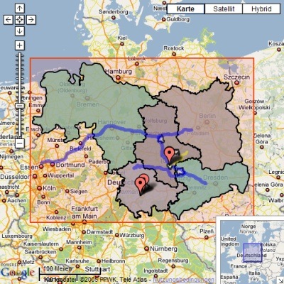
Die interessanteste Erkenntnis für mich war, dass mySQL in der aktuellen Version schon einen ausführlichen Support für Geometriedaten und Geometriefunktionen bietet. Das habe ich bisher nicht bemerkt, da mein myphpAdmin diese Datentypen und Funktionen nicht kennt und deshalb nicht anzeigt. Neben der Umrechnung und komprimierten Speicherung von Geoinformationen kann mySQL z.B. auch berechnen, ob sich zwei Polygone schneiden.
Im SQL Server 2008 wird im Zusammenhang mit Geoinformationen übrigens auch eine ganze Menge getan. Wer Interesse daran hat, kann sich zum Beispiel einen kurzen Webcast dazu ansehen.
Tags:
Geometrie,
GIS,
Google Maps,
mySQL,
SQL Server 2008
Thursday, 11. October 2007
Oct 11
“Was ist 2 mal 2 ?”
Der Ingenieur (zückt seinen Taschenrechner, rechnet ein bißchen…): “3,999999999”
Der Physiker: “In der Größenordnung von ein mal 10 hoch eins.”
Der Mathematiker (verzieht sich einen Tag in seine Stube, kommt dann freudestrahlend mit einem dicken Bündel Papier an): “Es existiert eine Lösung, und sie ist eindeutig!”
Der Psychiater: “Weiß ich nicht, aber gut, daß wir darüber geredet haben…”
Der Buchhalter (schließt alle Türen und Fenster und sieht sich vorsichtig um): “Was für eine Antwort wollen Sie hören?”
Der Jurist: “4, aber ich weiß nicht, ob wir vor Gericht damit durchkommen.”
Der Politiker: “Ich verstehe ihre Frage nicht…”
Der Mediziner: “4” – Alle anderen: “Pffft! Auswendig gelernt!”
Tags:
universität,
witze
Monday, 16. April 2007
Apr 16
Die mathematische Projektarbeit zur Fisher-Gleichung von Matthias Enders, Sebastian Wolf und Steffen Forkmann ist ab jetzt zum Download verfügbar. Hier ein Auszug aus der Einleitung:
“Die Fisher-Gleichung, auch als Kolmogorov-Petrovsky-Piscounov-Gleichung (KPP- Gleichung) bezeichnet, wurde im Jahre 1937 von Andrei Nikolaevich Kolmogorov (1903-1987) und Sir Ronald Aylmer Fisher(1890-1962) unabhängig voneinander untersucht.
Fisher nutzte sie, um die Ausbreitung eines vorteilhaften Gens innerhalb einer Population zu beschreiben. Die Gleichung vereint logistisches Wachstum mit einem Diffusionsterm in einer partiellen Differentialgleichung. Neben der Beschreibung von chemischen Reaktionen wird die Fisher-Gleichung heute vor allem dazu genutzt, die Invasion einer oder mehrerer Spezies in ein neues Gebiet zu modellieren.
Dieses Thema ist in der heutigen globalisierten Welt von großer Bedeutung, da durch den hohen Waren- und Personenverkehr immer öfter Organismen in vollkommen fremde Habitate eingeschleppt werden. Diese sogenannten Neobiota können bei fehlenden natürlichen Feinden weitreichende ökonomische und ökologische Schäden anrichten, wie aktuelle aber auch historische Beispiele zeigen.
Das wohl bekannteste Beispiel ist die Kaninchenplage in Australien, welche große Schäden in der Agrarwirtschaft verursacht hat. Das Aussetzen von nur 24 Kaninchen zu Jagdzwecken führte nach kurzer Zeit zu einer massiven Vermehrung der Kaninchen über den gesamten Kontinent. Aufgrund der Schwere der Massenvermehrung und den dramatischen Ernteverlusten wurde zwischen 1901 und 1908 sogar ein über 3000 km langer kaninchensicherer Schutzzaun (“Rabbit-Proof-Fence”) gebaut.
Als weiteres Beispiel für invasive Arten sei die aus Afrika stammende “Gelbe Spinnerameise” (Anoplolespsis gracilipes) gennant, die auf der Weihnachtsinsel im Pazifik innerhalb von nur eineinhalb Jahren circa drei Millionen Krabben getötet hat und den Fortbestand dieser und einiger anderer Arten akut bedroht.”
Im weiteren geht es um die mathematische Modellierung, die Analysis und die Simulation der Fisher-Gleichung.
Tags:
Mathematik
Sunday, 17. December 2006
Dec 17
Morgen werde ich zusammen mit Matthias Enders und Sebatian Wolf einen Vortrag über die Fisher-Gleichung halten. Die Fisher-Gleichung beschreibt ein mathematisches Modell mit dem man die Ausbreitung invasiver Arten beschreiben kann. Dieser Teil geht um die mathematische Analysis der Fisher-Gleichung – einige Simulationen werden später folgen.
Weitere Informationen gibt es auch in einem Artikel über die Modellierung biologischer Invasionen mit Reaktions-Diffusionsgleichungen von Ba Kien Tran.
Tags:
fisher-gleichung,
Mathematik